Structure

In the GitHub repository, the Seismo-VLAB's folder structure is organized in three directories:

• The 01-Pre_Process directory is divided in four sub-folders:
  • The Core folder provided with two main python files: SeismoVLAB.py that loads all required modules to generate a model; and Definitions.py that contains the data structure (dictionaries) that stores the finite element information. Also, Python routines provided in SVL handles the degree-of-freedom numbering in Numberer.py, the domain partition in Partition.py, soil spatial variability in RandomField.py, and domain reduction forces in PlaneWave.py. Other features can be incorporated to meet the user's need as well.
  • The Method folder provided with the python scripts Attach.py and Remove.py that allows to add/remove components in the Entities dictionary. It also provides with builder.py to generate simple domains in 1D, 2D, and 3D and discretize it. Similarly, several domains can be merged to generate more complex models, and they can be display using Display.py functions in ParaView software.
  • The Metis folder has a compiled version of the Metis software for different platforms (Linux, MacOS, and Windows). The Metis software is employed to generate the domain decomposition which is employed in Seismo-VLAB to perform a parallel execution. Basically, the model domain (i.e., group of objects such as Node, Element, Material, Section, and Load) is divided so that the number of elements are almost uniform across processors. Metis is called from the function SetMetisInputFile() defines in Partition.
  • The Parser allows the user to import a model generated from some software. The idea is essentially to load different models from different files and then tie them together using kinematic constraints. This will allow the user to generate complex interaction as the one required in SSI. The Parser function returns a mesh dictionary, therefore for this mesh to be assign to Entities in SVL.
• The 02-Run_Process directory is divided in twelve sub-folders:
  • The 01-Node folder includes the C++ Node and Constraint definition and declarations.
  • The 02-Materials folder contains the C++ definitions for Linear and NonLinear material.
  • The 03-Sections folder contains the C++ definitions for Plain and Fiber sections.
  • The 04-Elements folder is divided according to the element geometry into: ZeroLength, Links, Truss, Frame, Triangle, Quadrilateral, Membrane, Shell, Tetrahedron, and Hexahedron.
  • The 05-Loads folder includes the C++ Load and LoadCombo definition and declarations.
  • The 06-Mesh folder includes the C++ Mesh definition and declarations.
  • The 07-Assembler folder includes the C++ Assembler definition and declarations.
  • The 08-Analysis folder contains the derived classes for Static and Dynamic analyses.
  • The 09-Algorithms folder contains the derived classes for Linear and Nonlinear solution of the system of equations.
  • The 10-Integrators folder contains the derived classes for Explicit and Implicit time integration schemes.
  • The 11-Solvers folder contains the derived classes for Direct and Iterative solvers.
  • The 12-Utilities folder contains the classes for parsing the json input file as well as the recorder class.
• The 03-Validations directory is divided in three sub-folders:
  • The 01-Debugging folder contains a set of examples designed to check if basic features (Material, Section, Element, Algorithm, Integrator, and others) implemented in SVL work properly.
  • The 02-Performance folder contains a set of examples designed to check if the parallel features implemented in SVL works properly.
  • The 03-Report folder that contains a python script that runs all the debugging cases and generates a PDF report with results.

Inside the previous directories, the Seismo-VLAB's program files are provided and they are essential to run the two processes:

• The Pre-Analysis based on a Procedural Programming Paradigm.
• The Run-Analysis based on a Object-Oriented Programming Paradigm.

In general, as it will be discussed later, the Pre-Analysis can be totally omitted as long as the files required to run the Run-Analysis are provided in JSON format. More details are presented below.

Pre-Analysis

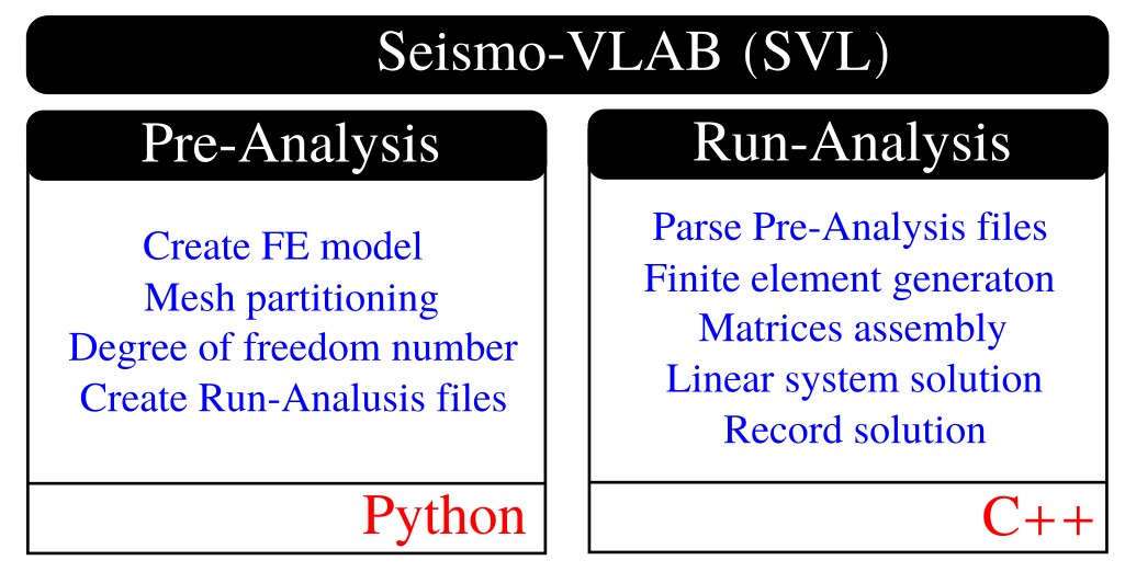
The Pre-Analysis consists on a set of Python routines that allows to construct a finite element model. This interface is designed to be user friendly and to handle large models in different formats. The main task is orchestrated by two scripts: 01-Pre_Process/Core/SeismoVLAB.py that essentially loads all required modules to generate a model; and 01-Pre_Process/Core/Definitions.py that contains the data structure (dictionaries) that stores the finite element information to be transformed into Run-Analysis input files.

A normal Pre-Analysis execution diagram is illustrated in the following figure:

As it is shown, the Pre-Analysis starts running the Script.py file and ends generating the File.#.$.json output files (where .$. token represents the processor number while the .#. token represents the load combination identifier). During this process the Pre-Analysis handles the degree-of-freedom numbering in 01-Pre_Process/Core/Numberer.py, the domain partition in 01-Pre_Process/Core/Partition.py, soil spatial variability in 01-Pre_Process/Core/RandomField.py, and domain reduction forces in 01-Pre_Process/Core/PlaneWave.py.

The Pre-Analysis also allows the user to parse formats from other softwares. For example, ETABS (.e2k), SAP (.s2k), and GMSH (.mesh) are currently available. Basic features such as node, material, element, restriction are transformed into SVL format, but they can be manipulated using Python to include other features as well. The Pre-Analysis also offers several routines that are provided in the 01-Pre_Process/Method/Attach.py that allows the user to create/append new entities using a Python interface. Then, a user can take full advantage of all the features available in Python to manipulate, modify and create more sophisticated finite element model.

Attention

The SVL Pre-Analysis modules are discussed in further details at Modules

Run-Analysis

The Run-Analysis is a C++ program that forms the main core of SVL. This process is in charge of generating the finite element model and performing the desired analysis. The Run-Analysis essentially generates the finite element matrices, assembles the contribution of each elements, and solves the resulting systems of equations to finally provided with the desired simulation results.

The Run-Analysis classes are stored in different folders so that the internal structure is better defined. For example, in the folders: 02-Run_Process/01-Node, 02-Run_Process/02-Materials, 02-Run_Process/03-Sections, 02-Run_Process/04-Elements, 02-Run_Process/05-Loads, and 02-Run_Process/06-Mesh the user will find all required classes to construct a finite element model. Similarly in folders such as: 02-Run_Process/08-Analysis, 02-Run_Process/09-Algorithms, 02-Run_Process/10-Integrators, and 02-Run_Process/11-Solvers contains all classes required to perform modifications on the finite element mesh.

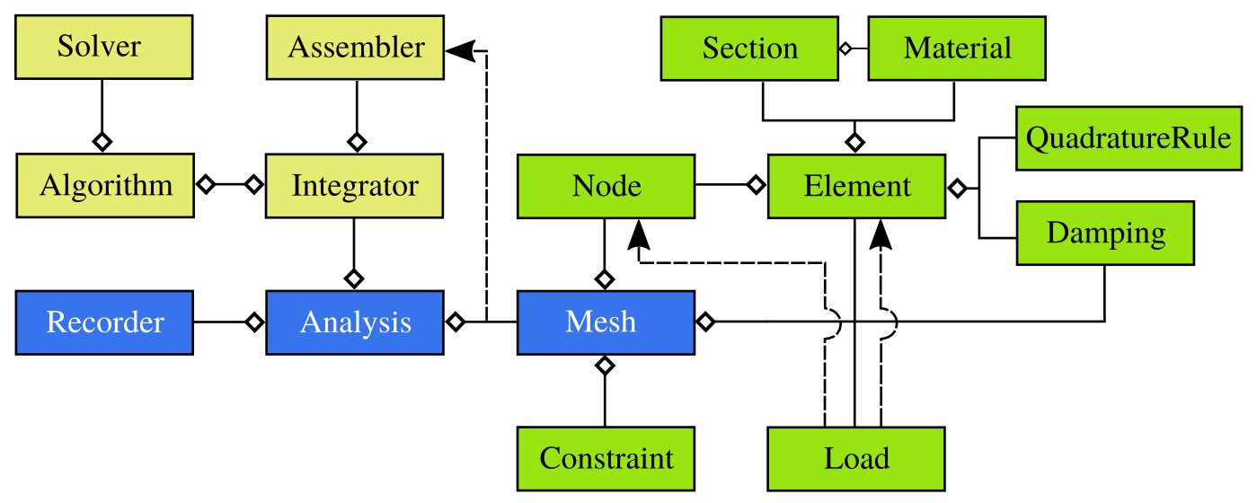
The Run-Analysis classes and their interaction are shown in the figure below:

The figure above shows the main abstract classes employed to develop the Run-Analysis. In this diagram, the diamond arrow that arrives at an abstract class represents an internal relation between them, for example the Element class is formed by Node and Material. The point arrow that arrives at an abstract class represents a dependency between them, for example a Load is given to an Element to compute external forces. The diagram represents in blue boxes the main classes (core) of the Run-Analysis, classes represented in green boxes forms the geometry module, while classes represented in yellow forms the analysis module.

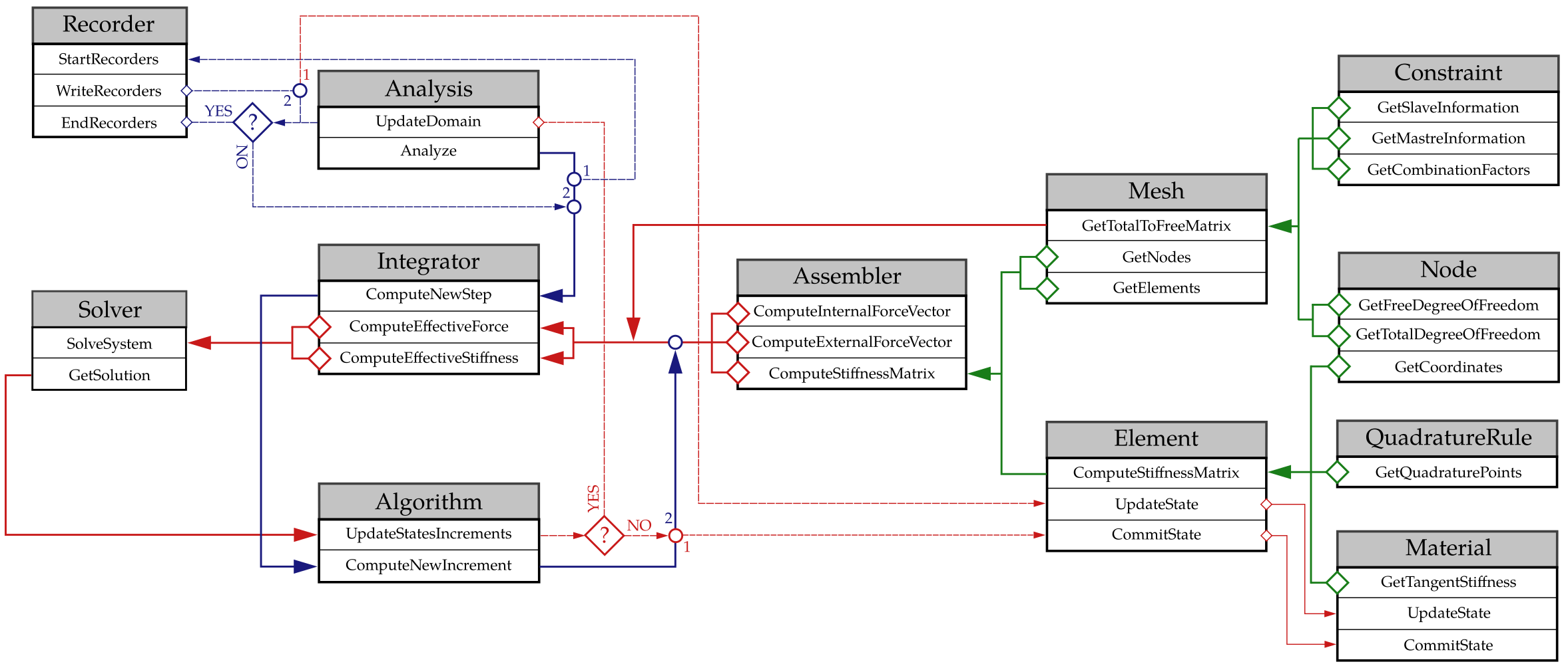
The Run-Analysis class diagram is illustrated in the following figure:

The flowchart starts at execution of the public member function Analysis::Analyze(). After this execution, the Recorder is immediately initialized using Recorder::Initialize. Then, the Integrator::ComputeNewStep() is called for each time step during the simulation. In each time step, the Algorithm::UpdateStatesIncrements() member is called. Inside this function, the effective stiffness matrix and force vector are computed using the Assembler. The Assembler asks the Mesh to provide with all Element and Nodes so that the Element::ComputeStiffnessMatrix() and Element::ComputeInternalForces() are for instance computed at each Element. The Element contribution is thus assembled into the global stiffness matrix and force vector. These quantities are passed to the Solver to obtain the solution of the linear system. The solution is retrieved in the Algorithm and used to update the incremental displacement at the public member function Algorithm::UpdateStatesIncrements(). Here, a convergence test is performed:

• If the state increment does not reach a certain tolerance, then the displacement increment is updated, and the Element::CommitState() is performed. A new iteration is performed (right after the states have been updated) until convergence is reached.
• If the tolerance is reached, then the domain is updated at StaticAnalysis::UpdateDomain() or DynamicAnalysis::UpdateDomain(), and the Recorder::WriteResponse() is called so that the states at this time step are stored.

Finally, after the domain has been updated, if the simulation reaches the last time step, then the Recorder::Finalize() is executed and the simulation is terminated, otherwise a new time step is computed.

Attention

The SVL Run-Analysis modules are discussed in further details at Modules

The Workflow

In general, SVL involves two independent execution:

• First, the Pre-Analysis (generation) is executed as:

  python3 '/path/to/Script.py'

• Second, the Run-Analysis (simulation) is executed as:
  • One processor (single core)
    

    /path/to/SeismoVLAB.exe -dir '/path/to/Partition/Folder' -file 'File.#.$.json'

  • Multi Processor (many core)
    

    mpirun -np n /path/to/SeismoVLab.exe -dir '/path/to/Partition/Folder' -file 'File.#.$.json'

The communication or link between the Pre-Analysis and the Run-Analysis is done through input and output file as shown below.

The generated input and output files during a SVL execution are:

• ./Script.py : Main python file (generated by the user) employed to create the finite element model. The Pre-Analysis python file is described in Modules. We insist on this process can be skipped as long as the File.#.$.json is written in Run-Analysis format.
• ./Partition/File.#.$.json : Set of partitioned input files generated in Pre-Analysis and written in Run-Analysis json format. Note that the .$. represents the processor number while .#. the load combination number. Each one of these files contains a subdomain of the finite element model.
• ./Solution/Response.out : Output files specified by the user that include Element, Node, Material, or Section responses.
• ./Paraview/Animation_PART$.n.vtk : These are VTK output files that can be displayed using ParaView. In the output file format $ represents the partition number and n the iteration or time step.

We have decided to generate the Mesh partitions and the degree of freedom numbering off-line using the Pre-Analysis. This allows Seismo-VLAB to be run almost fully parallel, avoiding the user to make mistakes by partitioning the domain manually. The Mesh partition can be easily checked using ParaView after executing the Pre-Analysis. This information is stored in the File.#.$.json files that are loaded in the Run-Analysis (using the function renderData() located at 01-Pre_Process/Method/Display.py).

Attention

The Pre-Analysis can be fully replaced by another program as long as the output files (./Partition/File.#.$.json) are written using the Run-Analysis json format.

The structure of the JSON format are discussed in Geometry Module, Solution Module, and Input/Output Module in the Run-Analysis section for more details.