Dynamic point-load

Background

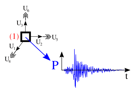
Represent a vector that is applied on a Node object. This force is represented by a magnitude that changes in time and direction. The Load object created in this manner is assembled directly to the global force vector, thus its direction must coincide with the global coordinate system.

REFERENCE:

• Bathe K. Jurgen, "Finite Element Procedures", Chapter 4: pages 161-166, Table 4.3, Prentice-Hall, 1996.

Pre-Analysis

The python Pre-Analysis in the 01-Pre_Process/Method/Attach.py file provides with an interface to create a DYNAMIC POINT LOAD. For example, to create a Dynamic point-load using json format, use:

• addLoad(tag, name='PointLoad', attributes):

  • tag : The identifier of this load, i.e., tag > -1
  • name : The Seismo-VLAB load class name, in this case: 'PointLoad'.
  • attributes : Specific properties for the PointLoad, for example
    • 'fun': The function identifier
    • 'list': The identifier of the nodes where this load acts upon
    • 'type': The type of load, in this case: 'Concentrated'.

  Example

  A DYNAMIC POINT LOAD can be defined using the python interface as follows:
  SVL.addLoad(tag=1, name='PointLoad', attributes={'fun': 1, 'type': 'Concentrated', 'list': [1]})

The information required to define the magnitude and direction of this Load is provided in the attributes['fun'] identifier. Thus, to create a DYNAMIC FUNCTION using the json format, use:

• addFunction(tag, name, attributes):

  • tag : The identifier of this function, i.e., tag > -1
  • name : The Seismo-VLAB function class name, in this case 'TimeSeries'.
  • attributes : The dynamic function information
    • 'dir' : The direction of the acting function
    • 'file' : The file where the load is going to be loaded. The file location is with respect to the main python script being executed

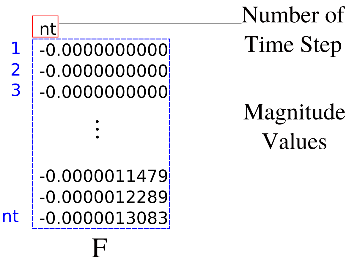
  The file format specified at attributes['file']='PointLoad.txt' must have the structure shown in the figure:

  

  Example

  A DYNAMIC FUNCTION can be defined using the python interface as follows:
  SVL.addFunction(tag=1, name='TimeSeries', attributes={'file': 'PointLoad.txt', 'dir': [0.0, 0.0, -1.0, 0.0, 0.0, 0.0])
  

Application
Please refer to the D16-DY_Free_Rectangular_3DPointLoad_Elastic_Frame2.py file located at 03-Validations/01-Debugging/ to see an example on how a DYNAMIC POINT LOAD and a DYNAMIC FUNCTION are defined.

On the contrary, the 01-Pre_Process/Method/Remove.py file provides with an interface to depopulate the Entities dictionary. For example, to remove an already define Load, use:

• delLoad(tag):
  • tag : The identifier of the load to be removed, i.e., tag > -1

Now, to remove a already defined function, use:

• delFunction(tag):
  • tag : The identifier of the function to be removed, i.e., tag > -1

Run-Analysis

The C++ Run-Analysis in the 02-Run_Process/05-Loads/Load.cpp file provides the class implementation. A DYNAMIC POINT LOAD is defined inside the "Loads" json field indicating its "Tag" as follows,

• {
      "Loads": {
          "Tag": {
              "name" : "POINTLOAD",
              "attributes": {
                  "name": "TIMESERIES",
                  "type": "CONCENTRATED",
                  "file": str,
                  "dir": [ ],
                  "list": [ ]
              }
          }
      }
  }
  

  Variable	Description
  Tag	Unique load object identifier.
  file	Represents the local address where the file is located.
  dir	Vector containing the direction of the force.
  list	List of Node identifiers that share this load.

  
  

  Attention

  The dimensions in dir must be consistent with the number of degree-of-freedom of that Node.

  The file provided in file for dynamic analysis contains the number of time steps, and then a vector with the varying intensities in time. The time step of such intensities is assumed to coincide with the time step of the simulation.

  Example

  A 2D DYNAMIC POINT LOAD applied downwards on node 2 whose intensities are located at ../Exterior.txt:
  { "Loads": { "1": { "name" : "POINTLOAD", "attributes": { "name": "TIMESERIES", "type": "CONCENTRATED", "file": "/full/path/to/folder/Exterior.txt", "dir": [0.000, -1.000], "list": [2] } } } }