Background

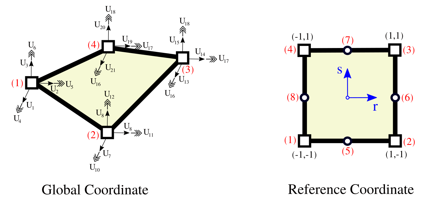
The lin3DShell4 class creates a linearized two-dimensional shell element with four-nodes. Each node has six degrees-of-freedom, for which three degree-of-freedom represent three translation in the X-, Y-, and Z-directions, and the other three rotation about the X-, Y-, and Z-directions. Figure provides a simple representation of this element in which the local coordinates are represented by the $r$-, $s$-, and $t$-axis, and (1), (2), (3) and (4) represent the nodes of the element respectively. The element mass, damping and stiffness matrices, as well as internal force vector are computed in local-coordinates and then transformed into global coordinates. Numerical integration is performed to compute matrices and vectors.

The isoparametric transformation has the advantage that every element is treated in the same manner. In this regard, mass and stiffness matrices as well as force vector are evaluated using the same reference coordinates as follows

\[ \mathcal{M}^\textrm{e} = \int_{-1}^1 \int_{-1}^1 {\textbf{N}^\textrm{e}_\textrm{m}} (r, s)^\top \, \rho^\textrm{e} \, \textbf{N}^\textrm{e}_\textrm{m}(r, s) \det \mathbf{J}^\textrm{e} \, dr \, ds + \int_{-1}^1 \int_{-1}^1 {\textbf{N}^\textrm{e}_\textrm{p}} (r, s)^\top \, \rho^\textrm{e} \, \textbf{N}^\textrm{e}_\textrm{p}(r, s) \det \mathbf{J}^\textrm{e} \, dr \, ds \,, \\ \mathcal{K}^\textrm{e} = \int_{-1}^1 \int_{-1}^1 {\textbf{B}^\textrm{e}_\textrm{m}} (r, s)^\top \, \mathbb{C}^\textrm{e}_\textrm{m} \, \textbf{B}^\textrm{e}_\textrm{m}(r, s) \det \mathbf{J}^\textrm{e} \, dr \, ds + \int_{-1}^1 \int_{-1}^1 {\textbf{B}^\textrm{e}_\textrm{p}} (r, s)^\top \, \mathbb{C}^\textrm{e}_\textrm{p} \, \textbf{B}^\textrm{e}_\textrm{p}(r, s) \det \mathbf{J}^\textrm{e} \, dr \, ds\,, \\ \mathcal{F}^\textrm{e} = \int_{-1}^1 \int_{-1}^1 {\textbf{N}^\textrm{e}_\textrm{m}} (r, s)^\top \, \textbf{F}_b^\textrm{e} \det \mathbf{J}^\textrm{e} \, dr \, ds \,, \nonumber \]

where $\rho^\textrm{e}$ is the element density, $\textbf{N}^\textrm{e}_\textrm{m}, \textbf{N}^\textrm{e}_\textrm{p}$ are the shape function matrix for the membrane and plate behavior, $\mathbb{C}^\textrm{e}_\textrm{m}, \mathbb{C}^\textrm{e}_\textrm{p}$ are the material constitutive law for membrane and plate behavior, and $\textbf{B}^\textrm{e}_\textrm{m}(r, s), \textbf{B}^\textrm{e}_\textrm{p}(r, s)$ are the well-known linear (material) strain-displacement matrix for the membrane and plate effects.

The mass and stiffness matrices as well as the force vector in global coordinates are defined as:

\[ \textbf{M}^\textrm{e} = \textbf{T}_\textrm{e}^\top \, \mathcal{M}^\textrm{e} \, \textbf{T}_\textrm{e} \,, \; \textbf{K}^\textrm{e} = \textbf{T}_\textrm{e}^\top \, \mathcal{K}^\textrm{e} \, \textbf{T}_\textrm{e} \,, \; \textbf{F}^\textrm{e} = \textbf{T}_\textrm{e}^\top \, \mathcal{F}^\textrm{e} \,, \]

In addition, the transformation matrix is

\[ \textbf{T}_\textrm{e} = \begin{bmatrix} \textbf{N} & 0 & 0 & 0 \\ 0 & \textbf{N} & 0 & 0 \\ 0 & 0 & \textbf{N} & 0 \\ 0 & 0 & 0 & \textbf{N} \end{bmatrix} \,, \; \text{ with } \textbf{N} = \begin{bmatrix} \hat{\textbf{N}} & 0 \\ 0 & \hat{\textbf{N}} \end{bmatrix} \,, \]

and $\hat{\textbf{N}} = [\hat{\textrm{n}}_1, \hat{\textrm{n}}_2, \hat{\textrm{n}}_3]^\top$ is the unit matrix of local coordinate axes, and $\hat{\textrm{n}}_\textrm{i}$ is the unit vector of the i-th local coordinate axis. Note that $\hat{\textbf{N}} \in \mathbb{R}^{3 \times 3}$, and $\hat{\textrm{n}}_\textrm{i} \in \mathbb{R}^3$. Note that $\textbf{M}^\textrm{e}, \textbf{K}^\textrm{e} \in \mathbb{R}^{\textrm{N}_\textrm{dof}^\textrm{e} \times \textrm{N}_\textrm{dof}^\textrm{e}}$ with $\textrm{N}_\textrm{dof}^\textrm{e} = 24$ in this case.

REFERENCE:

Adnan Ibrahimbegovic, "Quadrilateral finite elements for analysis of thick and thin plates", Computer Methods in Applied Mechanics and Engineering 110 (1993) 195-209.
Adnan Ibrahimbegovic, Robert Taylor, and Edward Wilson, "A Robust Quadrilateral Membrane Finite Element with Drilling degrees of freedom", International Journal for Numerical Methods in Engineering, vol. 30,445-457 (1990)

Pre-Analysis

The python Pre-Analysis in the 01-Pre_Process/Method/Attach.py file provides with an interface to populate the Entities dictionary. This file contains several functions to populate specific fields. For example, to create a lin3DShell4, using json format, use:

addElement(tag, name='lin3DShell4', conn, attributes):
- tag : The identifier of this element, i.e., tag > -1
- name : Seismo-VLAB element class name
- conn : Connectivity array of this element
- attributes : Specific properties for the created element, for example
  - 'section' is section identifier.
  - 'rule' the integration rule: 'Gauss', 'Lobatto'.
  - 'np' Number of quadrature-points used for the integration.
Example

A LIN3DSHELL4 element can be defined using the python interface as follows:
SVL.addElement(tag=1, name='lin3DShell4', conn=[1,2,3,4], attributes={'np': 9, 'rule': 'Gauss', 'section': 1})

Application
Please refer to the H03-ST_Lin_3DSlabPointLoad_ElasticPStress_Shell4.py file located at 03-Validations/01-Debugging/ to see an example on how to define a lin3DShell4 element.

On the contrary, the 01-Pre_Process/Method/Remove.py file provides with an interface to depopulate the Entities dictionary. For example, to remove an already define Element, use:

delElement(tag):
- tag : The identifier of the element to be removed, i.e., tag > -1

Run-Analysis

The C++ Run-Analysis in the 02-Run_Process/04-Elements/08-Shell/lin3DShell4.cpp file provides the class implementation. A lin3DShell4 element is created using the built-in json parse-structure provided in the Driver.hpp. A lin3DShell4 is defined inside the "Elements" json field indicating its "Tag" as follows,

{
    "Elements": {
        "Tag": {
            "name" : "LIN3DSHELL4",
            "conn" : [ ],
            "attributes": {
                "np": int,
                "rule": str,
                "section": int
            }
        }
    }
}

Variable	Description
`Tag`	Unique element object identifier.
`conn`	The element connectivity node array.
`np`	Number of quadrature-points used for the integration.
`rule`	The quadrature integration name `rule`=GAUSS, LOBATTO.
`section`	The section identifier.

Attention: This formulation allows small deformations.; Only one section is define at each integration point to compute this element.; Only linear biaxial material can be used in the section for this element.; Currently the number of integration points np= 1,4,9,16 are supported, another value assumes np=9.; The section thickness is assumed to be constant over the element and the same at each quadrature point.; The domain reduction force method is incompatible with this element.

Example

A LIN3DSHELL4 element between nodes 1, 2, 3 and 4, made of section 1 using with 9 integration points is constructed as:
{ "Elements": { "1": { "name" : "LIN3DSHELL4", "conn" : [1,2,3,4], "attributes": { "np": 9, "rule": "GAUSS", "section": 1 } } } }