Background

The kin2DQuad4 class creates a kinematic two-dimensional quadrilateral element with four-nodes. Each node has two degrees-of-freedom, and each degree-of-freedom represents a translation in the X-, and Y-directions. Figure provides a simple representation of this element in which the local coordinates are represented by the r-, and s-axis, and (1), (2), (3) and (4) represent the nodes of the element respectively. The element mass, damping and stiffness matrices, as well as internal force vector are computed in local coordinates and then transformed into global coordinates. Numerical integration is performed to compute matrices and vectors.

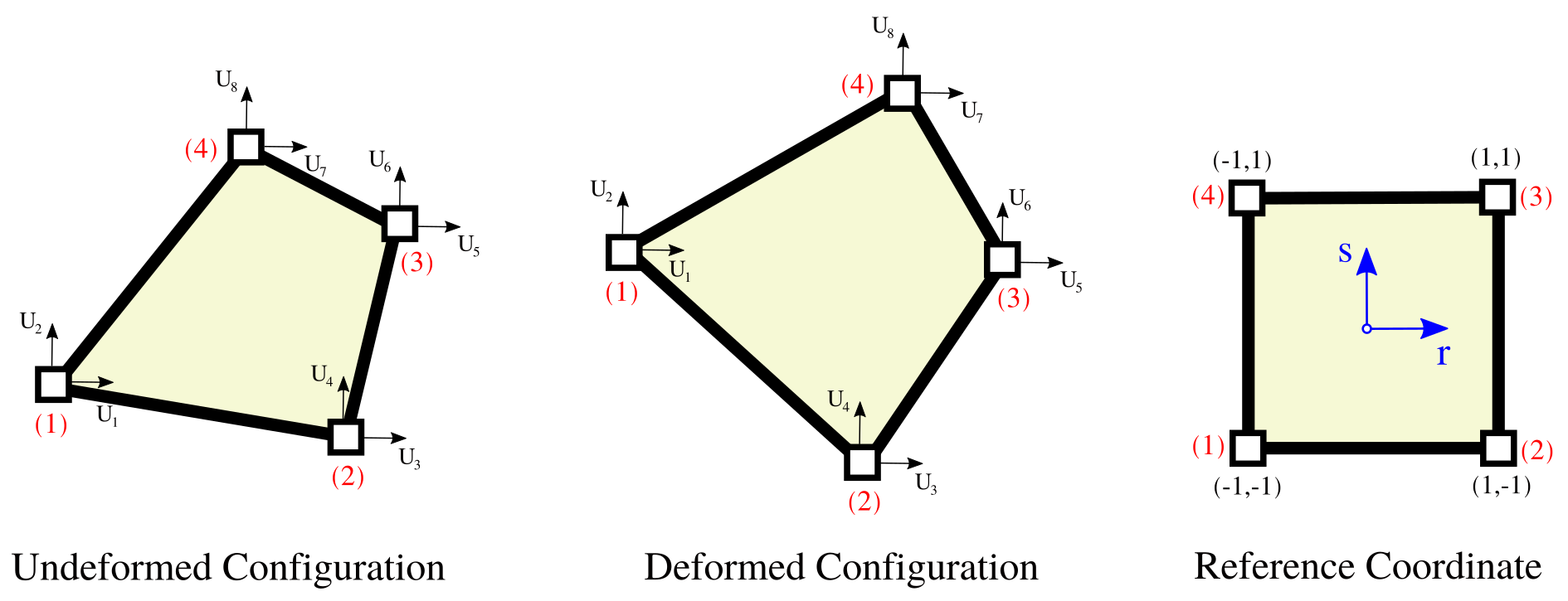
The undeformed configuration is represenented as \(X_1,X_2\), and the deformed coordinates of any point \(x_1,x_2\) in the element is written in terms of the shape functions \(\textbf{N}_\textrm{i}(r, s)\) in the reference coordinates as follows

\[ x_\textrm{j}^\textrm{e}(r, s ) = \sum_\textrm{i = 1}^{\textrm{N}_\textrm{n}} X^\textrm{(i)}_\textrm{j} \, \textbf{N}_\textrm{i}^\textrm{e}(r, s) \,. \nonumber \]

The same transformation is used to evaluate the displacements within the element–i.e., \(u_\textrm{j}^\textrm{e}(r, s)\). Then, the displacement field is approximated as

\[ u_\textrm{j}^\textrm{e}(r, s ) = \sum_\textrm{i = 1}^{\textrm{N}_\textrm{n}} u^\textrm{(i)}_\textrm{j} \, \textbf{N}_\textrm{i}^\textrm{e}(r, s) \,. \nonumber \]

Since both the displacement field and the point element coordinates are approximated using the same shape function, this formulation is commonly known as isoparametric transformation. Computation of the strain-displacement matrix \(\textbf{B}^\textrm{e}(x_1,x_2)\) now requires to be mapped into the reference coordinate systems. Application of the chain rule for differentiation to the shape functions yields

\[ \begin{bmatrix} \displaystyle{\frac{\partial N_\textrm{i}}{\partial r}} \\ \displaystyle{\frac{\partial N_\textrm{i}}{\partial s}} \end{bmatrix} = \begin{bmatrix} \displaystyle{\frac{\partial x}{\partial r}} & \displaystyle{\frac{\partial y}{\partial r}} \\ \displaystyle{\frac{\partial x}{\partial s}} & \displaystyle{\frac{\partial y}{\partial s}} \end{bmatrix} \begin{bmatrix} \displaystyle{\frac{\partial N_\textrm{i}}{\partial x}} \\ \displaystyle{\frac{\partial N_\textrm{i}}{\partial y}}\end{bmatrix} = \mathbf{J} \begin{bmatrix} \displaystyle{\frac{\partial N_\textrm{i}}{\partial x}} \\ \displaystyle{\frac{\partial N_\textrm{i}}{\partial y}} \end{bmatrix} \,, \nonumber \]

where \(\mathbf{J}: \mathbb{R}^2 \to \mathbb{R}^2\) is called the Jacobian matrix. Hence, derivatives in \(\textbf{B}^\textrm{e}(x_1,x_2)\) can be transformed into \(\textbf{B}^\textrm{e}(r,s)\) in the reference coordinates using the Jacobian matrix.

The four shape functions \(\textbf{N}_\textrm{i}^\textrm{e}(r, s)\) required to evaluate the shape function matrix \(\textbf{N}^\textrm{e}(r, s)\), the strain-displacement matrix \(\textbf{B}^\textrm{e}(r,s)\), and Jacobian matrix \(\textbf{J}^\textrm{e}(r,s)\) are:

\[ \textbf{N}_\textrm{1}^\textrm{e}(r, s ) = \frac{1}{4} (1 - r) (1 - s) \,, \nonumber \\ \textbf{N}_\textrm{2}^\textrm{e}(r, s ) = \frac{1}{4} (1 + r) (1 - s) \,, \nonumber \\ \textbf{N}_\textrm{3}^\textrm{e}(r, s ) = \frac{1}{4} (1 + r) (1 + s) \,, \nonumber \\ \textbf{N}_\textrm{4}^\textrm{e}(r, s ) = \frac{1}{4} (1 - r) (1 + s) \,. \nonumber \]

Knowing the Jacobian matrix, the deformation gradient can be computed as

\[ \mathbf{F} = \begin{bmatrix} \displaystyle{\frac{\partial x}{\partial X}} & \displaystyle{\frac{\partial x}{\partial Y}} \\ \displaystyle{\frac{\partial y}{\partial X}} & \displaystyle{\frac{\partial y}{\partial Y}} \end{bmatrix} \]

The isoparametric transformation has the advantage that every element is treated in the same manner. In this regard, mass and stiffness matrices as well as force vector are evaluated using the same reference coordinates as follows

\[ \textbf{M}^\textrm{e} = \int_{-1}^1 \int_{-1}^1 {\textbf{N}^\textrm{e}} (r, s)^\top \, \rho^\textrm{e} \, \textbf{N}^\textrm{e}(r, s) \det \mathbf{J}^\textrm{e} \, dr \, ds \,, \nonumber \\ \textbf{K}^\textrm{e} = \int_{-1}^1 \int_{-1}^1 {\textbf{B}^\textrm{e}} (r, s)^\top \, \mathbb{C}^\textrm{e} \, \textbf{B}^\textrm{e}(r, s) \det \mathbf{J}^\textrm{e} \, dr \, ds + \int_{-1}^1 \int_{-1}^1 {\mathcal{B}^\textrm{e}} (r, s)^\top \, \mathbb{S}^\textrm{e} \, \mathcal{B}^\textrm{e}(r, s) \det \mathbf{J}^\textrm{e} \, dr \, ds \,, \nonumber \\ \textbf{F}^\textrm{e} = \int_{-1}^1 \int_{-1}^1 {\textbf{N}^\textrm{e}} (r, s)^\top \, \textbf{F}_b^\textrm{e} \det \mathbf{J}^\textrm{e} \, dr \, ds \,, \nonumber \]

where \(\rho^\textrm{e}\) is the element density, \(\textbf{N}^\textrm{e}\) is the shape function matrix, \(\mathbb{C}^\textrm{e}\) is the material constitutive law, \(\mathbb{S}\) is the second Piola-Kirchhoff stress matrix, \(\textbf{B}^\textrm{e}(r, s)\) is the well-known linear (material) strain-displacement matrix, and \(\mathcal{B}^\textrm{e}(r, s)\) is nonlinear (geometric) strain-displacement matrix. Note that \(\textbf{M}^\textrm{e}, \textbf{K}^\textrm{e} \in \mathbb{R}^{\textrm{N}_\textrm{dof}^\textrm{e} \times \textrm{N}_\textrm{dof}^\textrm{e}}\) with \(\textrm{N}_\textrm{dof}^\textrm{e} = 8\) in this case.

REFERENCE:

Bathe, K. Jurgen, "Finite Element Procedures", Chapter 6: pages 549-55 (Table 6.5). Prentice-Hall, 1996.

Pre-Analysis

The python Pre-Analysis in the 01-Pre_Process/Method/Attach.py file provides with an interface to populate the Entities dictionary. This file contains several functions to populate specific fields. For example, to create a kin2DQuad4, using json format, use:

addElement(tag, name='kin2DQuad4', conn, attributes):
- tag : The identifier of this element, i.e., tag > -1
- name : Seismo-VLAB element class name
- conn : Connectivity array of this element
- attributes : Specific properties for the created element, for example
  - 'material' is material identifier.
  - 'rule' the integration rule: 'Gauss', 'Lobatto'.
  - 'th' is the thickness of a quad element.
  - 'np' Number of quadrature-points used for the integration.
Example

A KIN2DQUAD4 element can be defined using the python interface as follows:
SVL.addElement(tag=1, name='kin2DQuad4', conn=[1,2,3,4], attributes={'th': 0.01, 'material': 1, 'np': 4, 'rule': Gauss})

Application
This element has not been validated yet.

On the contrary, the 01-Pre_Process/Method/Remove.py file provides with an interface to depopulate the Entities dictionary. For example, to remove an already define Element, use:

delElement(tag):
- tag : The identifier of the element to be removed, i.e., tag > -1

Run-Analysis

The C++ Run-Analysis in the 02-Run_Process/04-Elements/06-Quadrilateral/kin2DQuad4.cpp file provides the class implementation. A kin2DQuad4 element is created using the built-in json parse-structure provided in the Driver.hpp. A kin2DQuad4 is defined inside the "Elements" json field indicating its "Tag" as follows,

{
    "Elements": {
        "Tag": {
            "name" : "KIN2DQUAD4",
            "conn" : [ ],
            "attributes": {
                "th": double,
                "np": int,
                "rule": str,
                "material": int
            }
        }
    }
}

Variable	Description
`Tag`	Unique element object identifier.
`conn`	The element connectivity node array.
`th`	The thickness of the element.
`np`	Number of quadrature-points used for the integration.
`rule`	The quadrature integration name `rule`=GAUSS, LOBATTO.
`material`	The biaxial material identifier.

Attention: This formulation allows large deformations.; Material non-linearity can be used in this element.; Currently the number of integration points np= 1,4,9,16,25,36,49 are supported, another value assumes np=4.; The material is considered to be the same at each quadrature point.; The domain reduction force method is compatible with this element.

Example

A KIN2DQUAD4 element of thickness 0.01 with 4 integration points between nodes 1, 2, 3 and 4, made of material 1 is constructed as:
{ "Elements": { "1": { "name" : "KIN2DQUAD4", "conn" : [1,2,3,4], "attributes": { "th": 0.01, "np": 4, "rule": "GAUSS", "material": 1 } } } }