Background

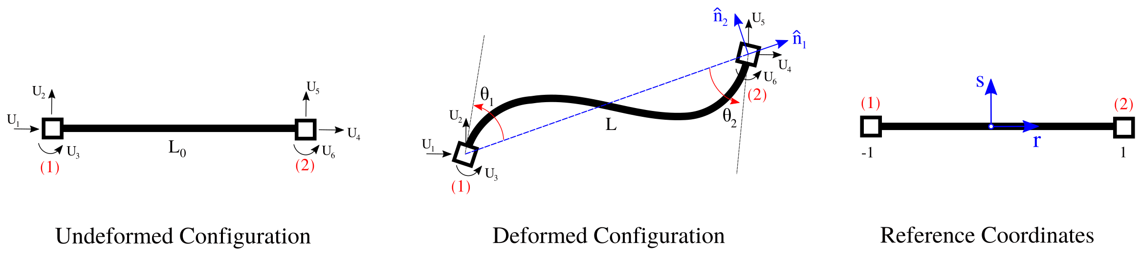
The kin2DFrame2 class creates a finite kinematic two-dimensional frame element with two-nodes. Each node has three degrees-of-freedom, for which two degree-of-freedom represents two translation in the X-, Y-directions, and one rotation in Z-direction. Figure provides a simple representation of this element in which the local coordinates are represented by \(\hat{\textrm{n}}_1\)-, \(\hat{\textrm{n}}_2\)-axis, and (1) and (2) represent the start and end nodes of the element, respectively. The element mass, damping and stiffness matrices, as well as internal force vector are computed in local-coordinates and then transformed into global coordinates. No numerical integration is employed for this element.

The kin2DFrame2 lumped and consistent mass matrix \(\textbf{M}^\textrm{e}\) in global coordinates are computed in the same manner as lin2DFrame2. On the other hand, the stiffness matrix is computed using a corrotational formulation.

In the corrotational formulation, the axial displacement \(u_\textrm{l}\) of the frame element is computed as

\[ u_\textrm{l} = \textrm{L} - \textrm{L}_\textrm{0} = \frac{\textrm{L}^2 - \textrm{L}_\textrm{0}^2}{\textrm{L} + \textrm{L}_\textrm{0}} \,, \]

where \(\textrm{L}\) is the frame length in the current configuration, and \(\textrm{L}_0\) the length in the initial configuration. Note that the last equality is to increase the condition of the subtraction.

Moreover, the bending moments developed at the end sections–i.e., Node (1) and (2) are computed as

\[ \textbf{M} = \begin{bmatrix} \textrm{M}_1 \\ \textrm{M}_2 \end{bmatrix} = \frac{2 \textrm{EI}}{\textrm{L}_0} \begin{bmatrix} 2 & 1 \\ 1 & 2 \end{bmatrix} \,. \]

The consistent tanget stiffness matrix is then computed as

\[ \textbf{K}^\textrm{e} = \textbf{T}_\textrm{e}^\top \textbf{K}^\textrm{e}_\textrm{m} \textbf{T}_\textrm{e} + \frac{\textrm{N}}{\textrm{L}}\mathbf{z}\mathbf{z}^\top + \frac{\textrm{M}_1 + \textrm{M}_2}{L} \left( \mathbf{r}\mathbf{z}^\top + \mathbf{z}\mathbf{r}^\top \right) \,, \]

where the matrix \(\textbf{K}^\textrm{e}_\textrm{m}\) is the material contribution obtained in lin2DFrame2, the vectors \(\mathbf{z} = [-\hat{\textrm{n}}_2^\top, \hat{\textrm{n}}_2^\top]\), and \(\mathbf{r} = [-\hat{\textrm{n}}_1^\top, \hat{\textrm{n}}_1^\top]\) are the variation of the global displacement vector. Note that \(\textbf{K}^\textrm{e} \in \mathbb{R}^{6 \times 6}\) and \(\mathbf{z}, \mathbf{r} \in \mathbb{R}^{3}\).

In addition, the local to global transformation matrix in current configuration is

\[ \textbf{T}_\textrm{e} = \begin{bmatrix} \hat{\textbf{N}} & 0 \\ 0 & \hat{\textbf{N}} \end{bmatrix} \,, \]

where \(\hat{\textbf{N}} = [\hat{\textrm{n}}_1, \hat{\textrm{n}}_2, \hat{\textrm{n}}_3]^\top\) is the unit matrix of local coordinate axes, and \(\hat{\textrm{n}}_\textrm{i}\) is the unit vector of the i-th local coordinate axis. Note that \(\hat{\textbf{N}} \in \mathbb{R}^{3 \times 3}\), and \(\hat{\textrm{n}}_\textrm{i} \in \mathbb{R}^3\). Note that \(\textbf{M}^\textrm{e}, \textbf{K}^\textrm{e} \in \mathbb{R}^{\textrm{N}_\textrm{dof}^\textrm{e} \times \textrm{N}_\textrm{dof}^\textrm{e}}\) with \(\textrm{N}_\textrm{dof}^\textrm{e} = 6\) in this case.

REFERENCE:

Louie L. Yaw, E. F, "2D Co-rotational Beam Formulation", Cross School of Engineering, Walla Walla University, November 30, 2009.

Pre-Analysis

The python Pre-Analysis in the 01-Pre_Process/Method/Attach.py file provides with an interface to populate the Entities dictionary. This file contains several functions to populate specific fields. For example, to create a kin2DFrame2, using json format, use:

addElement(tag, name='kin2DFrame2', conn, attributes):
- tag : The identifier of this element, i.e., tag > -1
- name : Seismo-VLAB element class name
- conn : Connectivity array of this element
- attributes : Specific properties for the created element, for example
  - 'section' is section identifier.
    Example
    
    A KIN2DFRAME2 element can be defined using the python interface as follows:
    SVL.addElement(tag=1, name='kin2DFrame2', conn=[1,2], attributes={'section': 1})
Application
Please refer to the D11-ST_kin_2DMomentBernoulli_Elastic_Frame2.py file located at 03-Validations/01-Debugging/ to see an example on how to define a kin2DFrame2 element.

On the contrary, the 01-Pre_Process/Method/Remove.py file provides with an interface to depopulate the Entities dictionary. For example, to remove an already define Element, use:

delElement(tag):
- tag : The identifier of the element to be removed, i.e., tag > -1

Run-Analysis

The C++ Run-Analysis in the 02-Run_Process/04-Elements/04-Frame/kin2DFrame2.cpp file provides the class implementation. A kin2DFrame2 element is created using the built-in json parse-structure provided in the Driver.hpp. A kin2DFrame2 is defined inside the "Elements" json field indicating its "Tag" as follows,

```
{
    "Elements": {
        "Tag": {
            "name" : "KIN2DFRAME2",
            "conn" : [ ],
            "attributes": {
                "section": int
            }
        }
    }
}
```
Variable Description

Tag Unique element object identifier.

conn The element connectivity node array.

section The section identifier.

Attention
This formulation allows large deformation and rotations.

Only one section can be used to define this element.

The section is assumed to be constant along the element.

The shear deformation is not included in this formulation.

The domain reduction force method is incompatible with this element.
Example

A KIN2DFRAME2 element between nodes 1 and 2, made of section 1 is constructed as:
{ "Elements": { "1": { "name" : "KIN2DFRAME2", "conn" : [1,2], "attributes": { "section": 1 } } } }

Variable	Description
`Tag`	Unique element object identifier.
`conn`	The element connectivity node array.
`section`	The section identifier.